Figures and export

Configure final and supporting figures, print active graphs, and export data, results, figures, and complete analysis reports.

Last verified: 2026-09-04

FT-ITC Analysis keeps publication figures, numerical data, and fitted result tables as separate output types. Final Figure is an Experiment Data workflow. An Analysis Result does not open directly as a Final Figure; Export Associated Final Figures... on a result exports figures for the experiment solutions associated with that result.

Final Figure

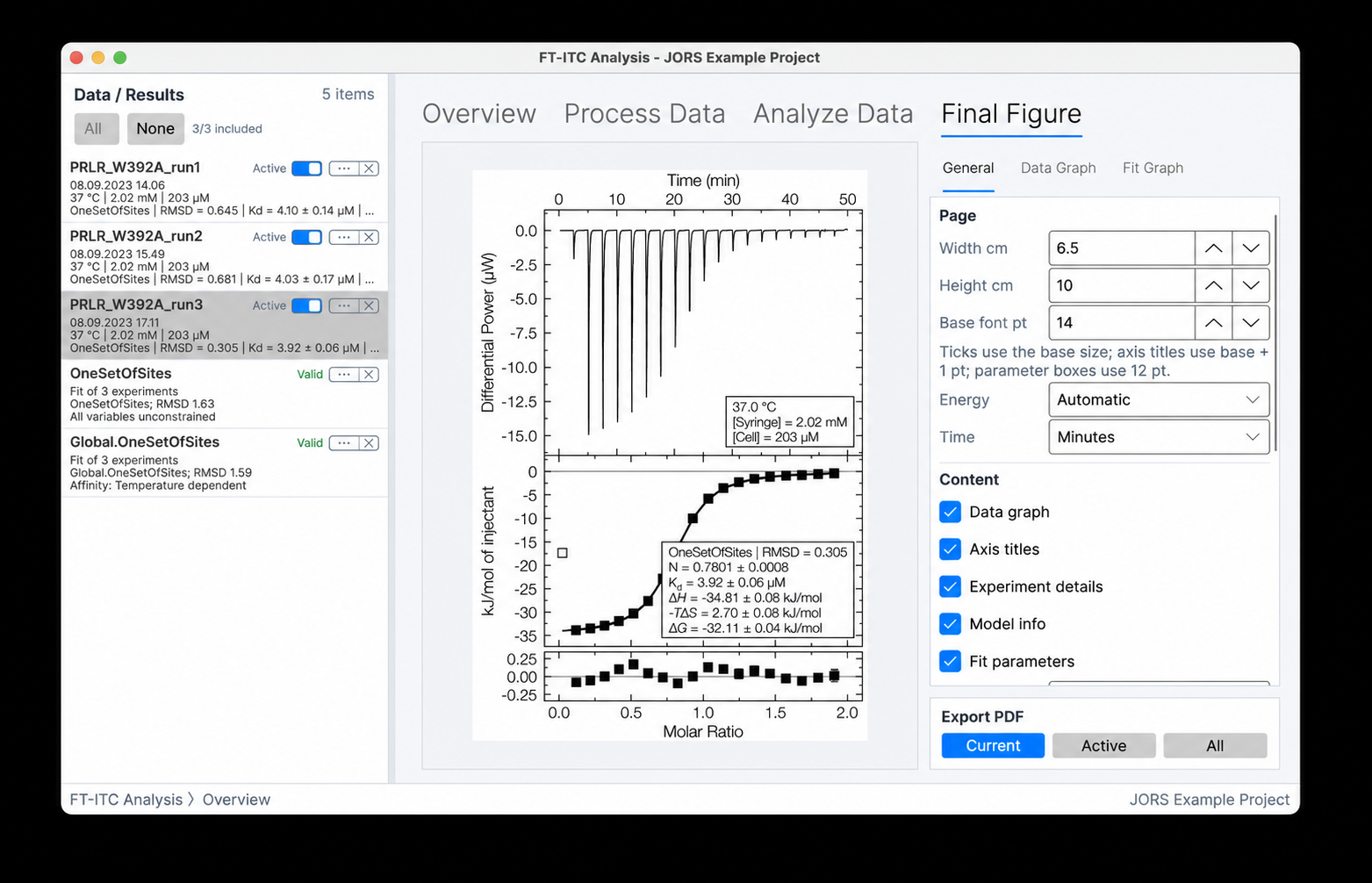
The Final Figure workspace renders the selected Experiment Data as a publication figure. Its preview and PDF output reflect the selected experiment, processing state, fitted solution, and figure options. An Analysis Result can supply fitted solutions for associated figure export, but the result itself is not the Final Figure workspace input.

The Export PDF controls contain three scopes:

• Current exports the displayed experiment figure to one PDF.
• Active exports figures for Active Experiment Data.
• All exports figures for all Experiment Data in the project.

The result-list command Export Associated Final Figures... loads the result’s member solutions into their experiments and writes one final-figure PDF per associated experiment. It is available for a result with exportable solutions. See Results and advanced analyses for result validity and stored member-solution behavior.

General

The General tab defines the page and common content. Page controls specify width and height in centimeters and the base font size. The Energy units selector provides Automatic, J, kJ, cal, and kcal. Automatic resolves one normal molar-energy unit from the figure's central plotted/result values; a fixed choice applies to all normal energy values. The selected family also controls thermogram units: differential power is µW or µcal/s, while integrated heat is µJ or µcal. Time controls set the displayed time unit. Content controls include the data graph, axis titles, experiment details, model information, fit parameters, and the information-box placement. The uncertainty selector provides Automatic, SD, CI, SD + CI, and None. Automatic uses the same per-quantity asymmetry rule described under Uncertainty and evaluation temperature.

The parameter controls determine which information appears in the information box: thermodynamic, derived, or offset parameters; temperature; concentrations; injection delay; instrument; and user-defined attributes. The information box is descriptive figure content and does not alter the underlying fit.

Data Graph

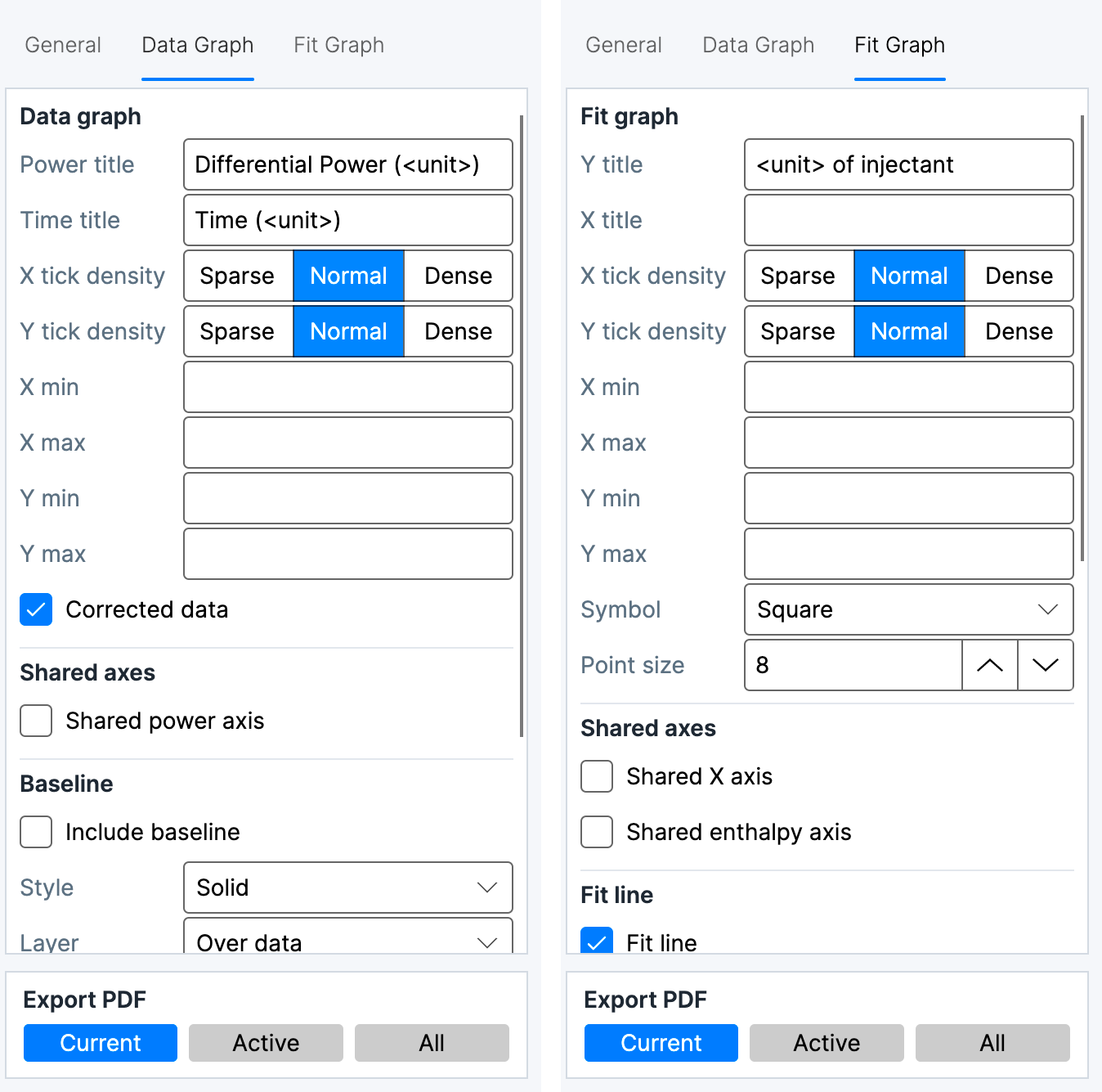
The Data Graph tab controls the differential-power trace. Power and time axis titles, tick density, and explicit minimum and maximum values define the axes. Corrected data selects the baseline-corrected trace when one is available. Shared power axis applies one power-axis range across the active experiments represented by a figure set.

Baseline controls expose the baseline, its Solid or Dashed style, Under data or Over data layer, and line width. Integration ranges displays the integration intervals as Bar, Fill, or Endpoint lines. These overlays describe processing and do not recalculate integration.

Fit Graph

The Fit Graph tab controls the integrated-heats and model panels. Enthalpy and molar-ratio axis titles, tick density, and explicit ranges define the axes. Symbols are Square or Circle, with an independent point size. Shared X axis and Shared enthalpy axis unify the corresponding ranges across active experiments; the residual-axis range follows the shared enthalpy setting when configured for unified residual axes.

Fit line displays the fitted binding curve with a selected width and Smooth, Spline, or Linear smoothness. Show residuals graph adds the residual panel, and Residual gap separates it visually from the fit panel. The display controls include the zero enthalpy line, confidence band, error bars, excluded points, excluded error bars, and offset-corrected heats. Error bars use processed injection uncertainties; confidence bands require bootstrap uncertainty in the fitted solution; fit lines and residuals require a fitted solution.

Numerical data export

File > Export Data... opens the numerical export dialog. Export Selected Data... invokes the same export for the selected experiment. The data scope is one of Selected experiment, Active experiments, or All experiments.

The format list contains:

• Thermogram Data — a .csv file containing time and power samples, with the Export baseline-corrected trace option when baseline-corrected samples exist.
• Integrated Peaks — a .csv file containing injection-axis values, integrated heats, uncertainties, fitted values, and residuals when available, with Export offset-corrected peaks when a fitted solution is available.
• Combined Data — a .csv file placing thermogram samples and integrated-peak columns side by side; raw, corrected, fitted, and residual columns are included when available.
• MicroCal / SEDPHAT — a .dat file with MicroCal-style DH, INJV, Xt, Mt, XMt, NDH, DY, and Fit columns. DH is in µcal, INJV is in µL, concentrations are in mM, and NDH, DY, and Fit are in cal/mol. The first injection uses -- for normalized heat and residual, following the conventional excluded-first-injection layout.
• pytc — a .dh file containing the pytc-compatible injection and metadata fields.
• ITCsim — a .csv file containing ITCsim-compatible injection data and metadata, with offset-corrected peaks available when a fitted solution exists.

Output units are format-specific. Thermogram samples use seconds and watts; integrated-peak and combined-data enthalpy, model, and residual values use joules per mole; MicroCal/SEDPHAT, pytc, and ITCsim use their documented concentration, volume, temperature, and heat conventions. The application energy-family preference controls desktop presentation, not these raw/scientific interchange contracts. Fitted columns and correction controls are disabled when the selected data do not contain the corresponding processed or fitted state. Export defaults are described in Settings and defaults.

These exports are not project backups. General .csv and .tsv exports cannot be reopened through File > Open.... A MicroCal / SEDPHAT .dat export or pytc .dh export can be reopened as integrated-heat input, but doing so restores neither a thermogram nor the FT-ITC project state and requires choosing the source heat unit. Select microcalorie for the DH column when reopening a newly generated MicroCal / SEDPHAT export. Historical FT-ITC .dat exports may instead require joule, matching the unit used when they were created. Save an .ftxtc project when the analysis must remain editable.

Analysis Result Exporter

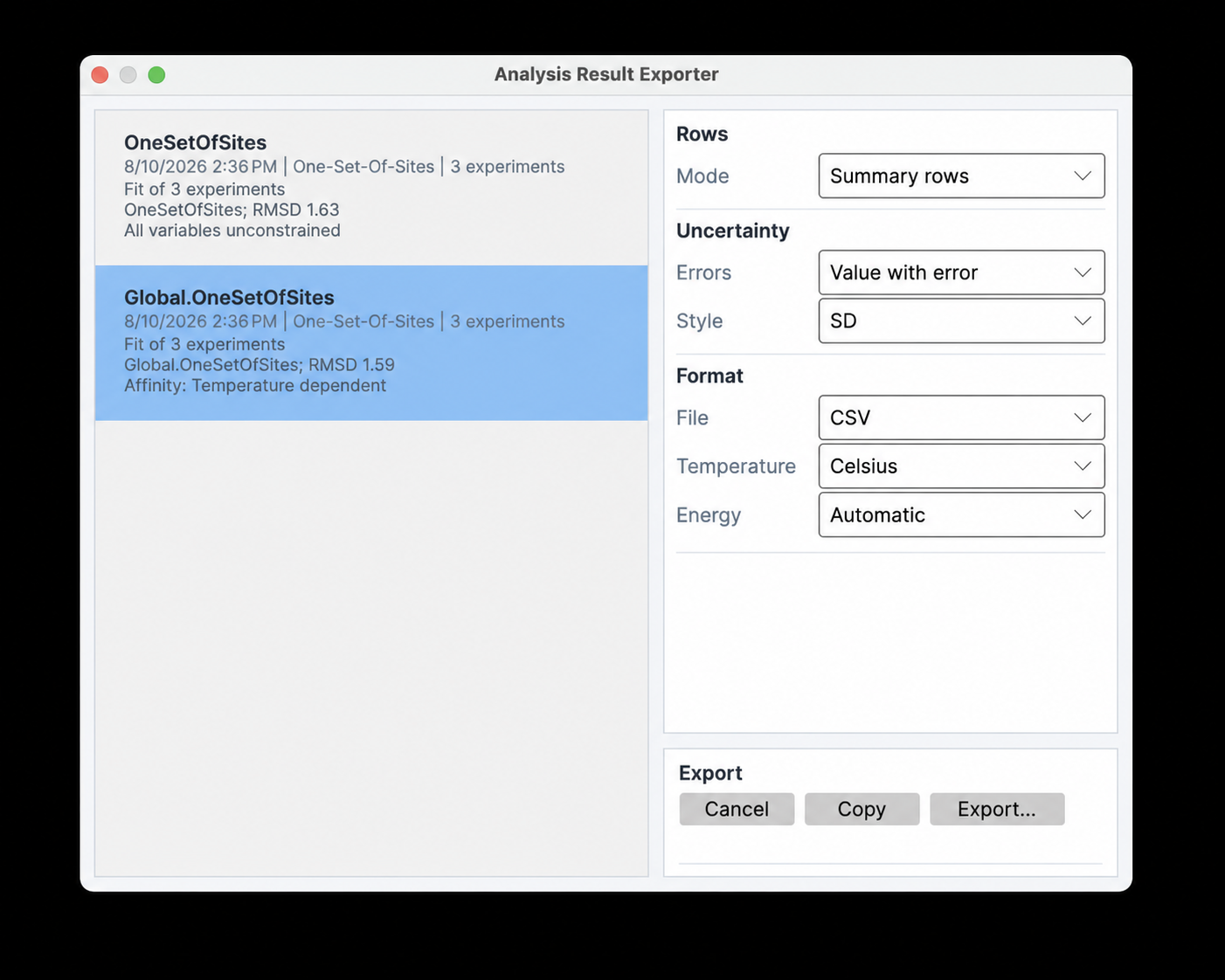
Analysis Result Exporter... builds a table from one or more selected Analysis Results. Summary rows emits result-level rows; All replicate rows emits the individual fitted/member rows. Error layout is Value with error or Separate columns. Uncertainty style is SD, CI, or SD + CI. The file format is CSV or TSV. Energy units provides Automatic, J, kJ, cal, and kcal. Automatic chooses one stable molar-energy unit across all selected results and one independent unit for ΔCp columns; a fixed choice applies its normal energy numerator consistently. Temperature presentation is Celsius or Kelvin.

The configured table is available through Copy and Export.... Copy places the same delimited text on the clipboard; Export writes it to a file. Profile-likelihood SD columns use the equivalent display scale implied by their stored endpoints and are labeled as such in exported metadata; the exact lower/upper endpoints remain available in separate-column mode. The exporter does not include the parameter-correlation matrix, which is calculated for display rather than stored as a result-table field.

Result tables, clipboard output, final-figure metadata, and viewer output create thermodynamic columns from the fitted model shape. A sequential result therefore exports one Kd, ΔH, ΔG, and −TΔS value for every active step, including steps 3 and 4, rather than truncating the result to two interactions. The fixed step count is included as model information. Values remain in their displayed families; exporting does not convert macroscopic sequential constants into microscopic site constants.

Each affinity column chooses its concentration unit independently from its own magnitude. For example, Kd1 may be shown in nM while Kd4 is shown in µM. The column header and its values always use the same unit; this is display scaling only and does not change fitted or persisted values.

Analysis Report

Tools > Analysis Report... creates a complete, printable report from one or more saved Analysis Results. The same tool is available as Export Analysis Report... in result-specific menus, where that result is initially selected. Use Select report contents... to choose results and optional supporting experiments together. The picker follows application order; applying the same ordered selection again restores its saved study context and approved interpretation. At least one result is required.

Report contents and layout

The report is a multipage A4 portrait PDF with margins suitable for printing. A report containing multiple results begins with a combined result index and concise table of contents on the first page, followed by the report-level interpretation and one self-contained chapter for each result. Results are referenced as 1, 2, and so on, and their experiments as 1A, 1B, 2A, 2B, and so on. These labels are derived from the saved result and experiment order, so figures, captions, and interpretation evidence use the same stable references. No experiments or scientific estimates are merged across results. Each chapter overview arranges the experiments in compact, borderless figure panels labeled with their references and names. The report automatically chooses three to five columns, centers incomplete rows, and suppresses repeated axis titles.

The analysis summary contains a compact grouped thermodynamic bar chart for every saved member and active binding step. Its whiskers show only the saved 95% confidence interval from the solution distribution or profile-likelihood calculation; the symmetric SD approximation remains available in report tables but is not superimposed on this plot. Each experiment section places a wider, baseline-focused view of the uncorrected thermogram—with its saved baseline and compact horizontal markers for the integration windows—beside a top-aligned Final Figure at its standard size containing the complete thermogram, followed closely by fitted and derived parameters. When Injection tables is selected, a table records every saved injection, its inclusion state, volume, concentrations, analysis-axis value, integrated heat and uncertainty, fitted heat, and residual. This processing presentation is an automatic report preset and does not add another figure control. A concise notice replaces the processing graph when raw thermogram samples are unavailable. Selected shared correlations follow the analysis summary; selected member correlations follow that experiment’s parameter table, using a compact native matrix rather than a dedicated page.

Directly selected experiments that are not represented by a selected result appear once in a report-level Supporting experiments chapter after the result chapters and are labeled S1, S2, and so on. The report uses only saved content: a raw thermogram with any saved baseline and integration boundaries, finite integrated heats explicitly labeled as having no fit, experiment metadata, notes about processing or correction exceptions, dates with a verified source, attributes, comments, and the report-wide optional injection table. Missing stages receive concise availability notices. Experiments already represented by a checked result remain visible but unavailable as supporting selections. Recorded buffer-subtraction references may be selected automatically according to the application setting, but remain ordinary optional selections; the report does not judge whether a reference is an appropriate blank. Report creation never fits, reintegrates, or performs subtraction.

Configure the report

Choose a title, an optional subtitle, energy and temperature units, and an Uncertainties style. The subtitle appears as secondary, regular-weight text below the report title. Reports default to SD + 95% CI. The selected style controls uncertainty in tables and applicable analysis plots. The thermodynamic summary bar chart always shows available saved 95% confidence intervals, as described above; it does not add SD whiskers. This selection is remembered only for the current application session. Final Figure injection errors and fitted confidence bands retain their established scientific meanings.

Optional content includes report-wide Injection tables and Condense repeated experiments switches and the completed analysis types available in any selected result. Each option applies to every eligible result chapter; chapters without that saved content simply omit it. The injection-table switch is on by default and applies consistently to every experiment. When the same experiment occurs in a later result, condensed mode retains both figures, comments, source file, date with a verified source, instrument, temperature, concentrations, and all result-specific fitted content, but replaces repeated secondary acquisition and processing details with a reference to its first occurrence. The Parameter correlations option includes the shared matrix and all available member matrices alongside their corresponding summaries. Available analyses are selected by default; Select all and Clear change that analysis list together. Temperature dependence is included once per eligible result with its saved fit and parameter summary, while saved electrostatics, protonation, and Spolar outputs are presented without recomputation. Report creation never reruns fitting or advanced analysis.

Write and preview an interpretation

The builder opens in Interpretation mode with an editor for your remarks. Text wraps automatically. Interpretation Markdown supports ## section headings, ### subsection headings, bullets, **bold**, and *italic* emphasis. Use the Interpretation / Preview control above the workspace to move between writing and the rendered report. Selecting Preview automatically builds the PDF when it has not yet been built or is out of date; a current preview is reused. Update Preview forces a rebuild. Editing while a preview exists marks it as out of date without repeatedly rendering while you type. Export PDF... rebuilds stale content and saves the completed PDF. Results with warnings, outdated inputs, or partially invalid status remain exportable and carry a prominent notice. A structurally unusable result shows a validation error and cannot be previewed or exported.

Generate an automated interpretation

Online generation privacy: Generate sends selected names, comments, conditions, fits and injection evidence, plus your question/context, to app.ft-itc.org (MIST), then OpenAI. Thermograms are off by default. MIST retains usage metadata without automatic expiry; full scientific payloads and generated prose are not stored in those usage tables. Provider and infrastructure retention are separate; no deletion deadline is guaranteed. Canceling does not retract sent data. Local processing, fitting, saving and export work without generation. Data flow and retention.

The inspector’s Interpretation section reports whether the text is manual, automatically generated, user edited, or out of date. Edit returns focus to the large editor. Generate interpretation… opens a dialog with optional Main question and Additional context fields. Use the question to focus the assessment and the context to explain the experiment. The cross-platform dialog labels its preset selector Interpretation depth. Requesting generation sends the selected report evidence and these inputs to the online interpretation service. Compressed thermograms are omitted by default to keep the model input compact. Administrators and Advanced capability-code users can opt in to Include compressed thermograms; standard and public access do not show the control.

Generation assesses all selected results and supporting experiments together, using the same references as the PDF. Results remain independent, including alternative fits of the same experiment. Supporting experiments contribute available observations and metadata without being assigned a fitted result or assumed control role. Generation uses existing processing, integration, residual, and uncertainty evidence where available; it does not rerun integration, baseline fitting, or model fitting. When compressed thermograms are included, they contain minimum and maximum power values for each 15-second interval, plus an aligned fitted baseline when available. Exact peak timing, the order of values within each interval, and the detailed waveform are unavailable. Oversized requests may omit complete traces while retaining summaries, injection tables, and fit evidence; these omissions are recorded.

When several result members have identical source data and processing, the request can share that evidence between them. Each result retains its own fitted values, uncertainty, validity, and constraints. Sharing source evidence does not imply independent replication or equivalent fits.

One warning allows you to review stale or failed analyses before continuing. Historical fit-input snapshots and stored estimates are distinguished from current observations; diagnostics requiring a verified matching fit basis are unavailable when that basis cannot be established. An interpretation can identify potential concerns, but it does not certify the experiment or establish a mechanism. Configured knowledge-base retrieval can support sparse paper-name, journal and year references; web search is disabled.

Review and edit the returned draft, then choose Use in report to replace the approved interpretation. The draft focuses on observed issues and targeted follow-up checks, using references such as Result 2 and Experiment 1B. It avoids routine warnings based solely on modest deviations in fitted N-values or missing blank titrations.

The interpretation service is asked to keep straightforward assessments to about 500–600 words or fewer, with roughly 1,000 words available for complex collections. These are writing targets, not acceptance limits. Longer text flows onto additional pages without automatic shortening or regeneration. Text length, headings, and Markdown formatting do not prevent you from accepting a draft.

Markdown tables require a header and separator row. They support bold or italic cell text and left, center, or right alignment. Cells wrap, and table headers repeat across pages. Use a few columns to keep tables readable. Unsupported formatting may appear as literal text in the report.

Canceling, closing the dialog, or encountering a service error leaves previously approved text unchanged. Study context, the thermogram setting, approved text, and generation details are saved with the report. Changes to selected results, supporting evidence, context, or settings can mark an approved automated interpretation as out of date. Older approved interpretations remain readable even when their freshness cannot be verified. The report distinguishes manually written interpretations from automatically generated text and subsequent edits.

The Summary generation task produces a compact factual report without knowledge-base retrieval or capability-code quota usage. Administrator access also provides a Scientific guidance selector for retained guidance revisions and an unchecked, per-request Omit scientific guidance experiment in the generation dialog. Omission removes the scientific guidance file but retains a minimal boundary that treats package and retrieved text as evidence, not instructions. Summary never permits omission. The generated draft and approved report provenance show the effective model, reasoning effort and guidance revision. Local report editing, saved interpretations, and PDF export remain available if automated interpretation generation is unavailable.

Save the interpretation package

Use Save package in the generation dialog to save a local ZIP containing the complete evidence (canonical-package.json), the compact model input (model-package.json), the application's output instructions, and a manifest of versions and instruction fingerprints. The export uses the current selection, question, context, and thermogram setting without contacting the service or running new fits. It captures the request before it is sent and does not include the service's scientific instructions. The archive contains your scientific data and context, so review it before sharing.

Use model-package.json to inspect the compact evidence prepared for model evaluation. Use canonical-package.json when you need full precision or all saved control-point details for auditing. The compact file keeps baseline diagnostics with each experiment. Landmark and spline-control arrays use tables with shared column definitions; spline-point locked, slopeLocked, and linear flags are omitted, while unknown point fields remain in an explicit extension map. Segmented-baseline tables retain boundaries, centers, injection scope, and complete coefficient arrays. Shared source evidence is stored under experimentEvidence; each member links to it through experimentEvidenceRef while retaining its own fit table.

Compressed traces use the uniform-minmax-v1 encoding: each 15-second interval stores a [min, max] power pair in µW relative to the trace offset. A start-time anchor and interval width specify timing. The pair gives the power range, not the chronological order of the samples. An independently calculated, aligned baseline array is retained when available.

Troubleshoot automated interpretation

Include the application log and the visible error when reporting a generation failure. The log records generation stages, request IDs, guidance revisions, instruction fingerprints, package sizes, timing, HTTP status, and rejected request or response fields. These diagnostic entries omit full instructions, scientific context, generated text, and credentials. An instruction fingerprint identifies a particular text but cannot reconstruct it.

The desktop app and interpretation service (MIST) must use the same relay contract, currently 6.0; the evidence package uses schema 2.0. MIST supplies scientific guidance, while the app supplies output instructions for its report renderer. The app and service do not negotiate compatibility automatically and must be updated together when the contract changes.

Choose the appropriate output tool

The Analysis Report is distinct from the other output tools:

• Analysis Result Exporter writes compact CSV or TSV tables for numerical reuse.
• Final Figure writes a publication figure for an experiment, while Export Associated Final Figures... writes one figure per result member.
• Supporting Figure composes selected figures into one multi-panel canvas.
• Analysis Report assembles one or more saved results as self-contained chapters with figures, detailed tables, diagnostics, optional advanced plots, and provenance.

Supporting Figure

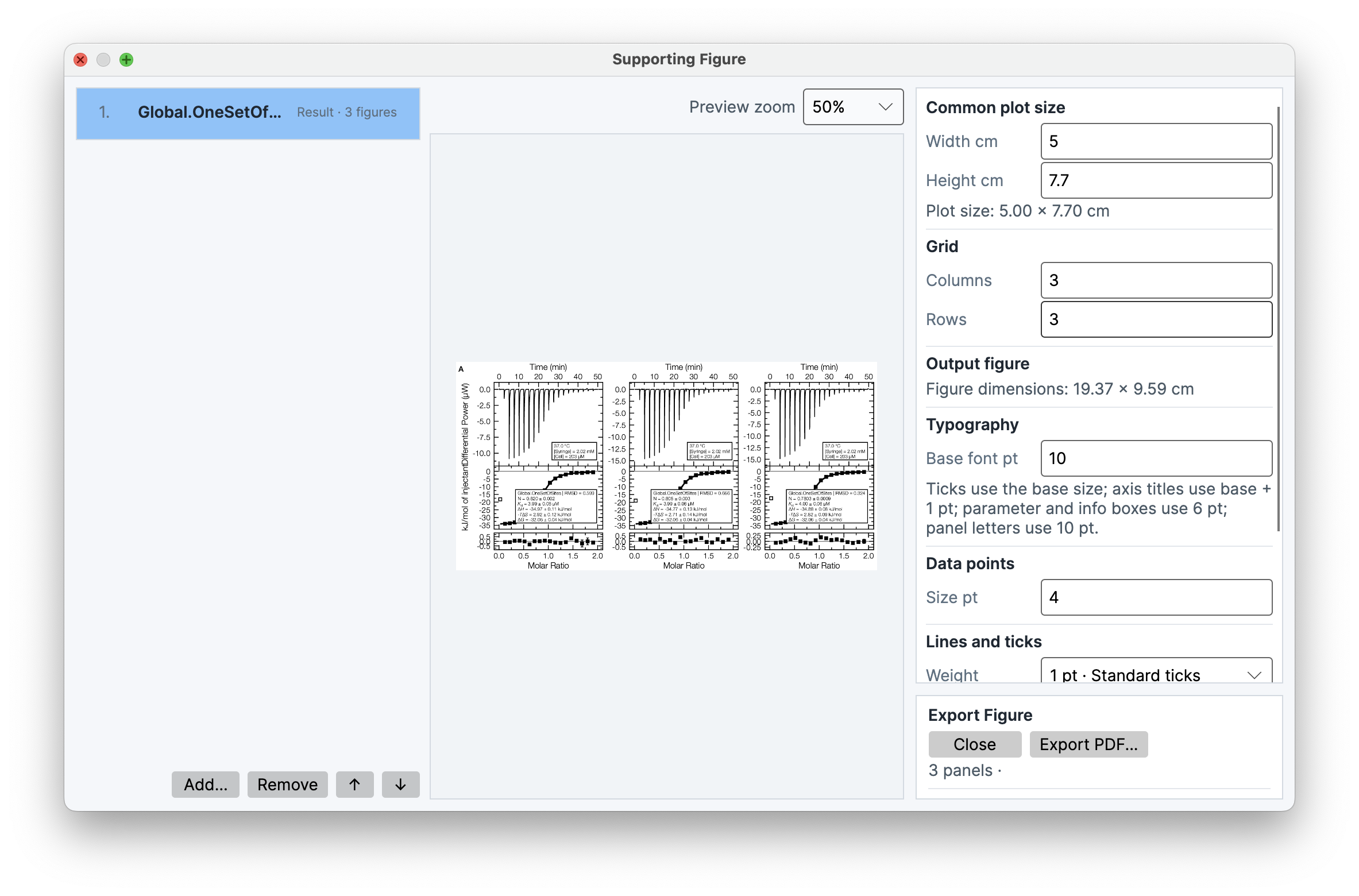
Supporting Figure... composes figures from Experiment Data and Analysis Results into a multi-panel canvas. The Figure order list defines source order; Add…, Remove, Up, and Down change the composition. The source picker can filter available experiment and result figures by name or type.

Common plot size specifies width and height in centimeters. Grid controls specify columns and rows. Typography controls define base font size, point size, line weight, and tick style. Panel letters adds stable A, B, … identifiers. Panel titles optionally adds the experiment name after that identifier (for example, A. Experiment name) and is off by default for existing Supporting Figure workflows. Group result figures and the parameter and information box control affect result grouping and annotations. The preview zoom shows the rendered canvas at 25%, 50%, 75%, or 100%. Export PDF... writes the composed supporting figure as a PDF.

Printing

File > Print prints the active graph or figure through the operating system’s print workflow. The active target can be the overview thermogram, processing graph, analysis graph, result graph—including an available Correlation matrix—or Final Figure, depending on the selected workspace. The operating-system print dialog supplies the available printer and PDF destinations; the graph content comes from the active application view.