
Quick start
Open your own ITC dataset, process it, fit a one-set-of-sites model, review the result, save the project, and export a figure.
Last verified:
This procedure takes a compatible file through an ordinary one-set-of-sites analysis. Use a dataset for which that model is scientifically plausible. The goal is to learn the application workflow, not to prescribe the correct model for every interaction.
Before you begin
Have one of these inputs available:
- a raw thermogram from a MicroCal-style file (
.itc), native TA Instruments NanoITC file (.nitc), NanoAnalyze export (.ta), or PEAQ-ITC project (.apj). - an Origin project file (
.opj). When a recognized ITC worksheet contains the original time/power trace, FT-ITC Analysis restores it for processing; otherwise, it uses the worksheet heat values as integrated input. - injection-level integrated heats (
.dat,.aff, or.dh). - an FT-ITC project (
.ftxtc).
Supported formats and project behavior are described in Installation, files, and projects.
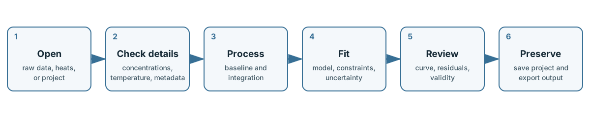
1. Open your data
Launch FT-ITC Analysis and choose Open File... on the welcome screen, choose File > Open..., or drag compatible files into the application window. Select your file and confirm the open operation.
The experiment appears in the data list. Select it and open Overview to orient yourself in the imported experiment. Drag any non-button area of a data or result row to change its position. This order is used throughout the application and is retained when the project is saved as .ftxtc.
2. Edit experiment details
Open Details... for the selected experiment. Concentration entries and the experiment date/time can be changed here when needed. Comments and attributes relevant to later analysis can also be added or edited. A changed date is marked as user-modified in the experiment overview.
Apply corrections only when you have an independent experimental basis. Concentration entries influence the calculated concentration ratio and fitted parameters.
3. Process a raw thermogram
If the import contains a thermogram, open Process Data.
- If the trace shows a smooth global drift, try Polynomial baseline. For more complicated baseline shapes, choose Spline; for local baseline behavior, choose Segmented. Keep the default integration settings initially.
- Inspect whether the baseline represents the signal between injections rather than the peaks.
- Inspect the start and end of every integration region. A region should include the injection response without extending unnecessarily into baseline noise. Zoom to a peak and adjust the integration end point. Use Space to copy the integration length to the next injection; the start is also copied when Copy start time to next is enabled.
These baseline alternatives are explained in Processing.
4. Fit one set of sites
Open Analyze Data, choose Single experiment, and select One-Set-Of-Sites.
- Review the initial parameter values. Use physically plausible orders of magnitude for affinity, enthalpy, and stoichiometry.
- Choose an optimizer. Levenberg-Marquardt is efficient near a suitable solution; Nelder-Mead can be useful when the starting surface is less cooperative.
- Optionally enable Weight by injection error when the integration uncertainties are meaningful for the dataset.
- Choose None, Bootstrap residuals, Leave-one-out, or Profile likelihood for error estimation.
- Choose Run Fit.
Create analysis result determines whether a usable fit also creates a separate Analysis Result. Enable it to continue through the result workspace in the next step; otherwise, the fitted solution remains attached to the Experiment Data.
If the fit fails or reaches a limit, the possible causes are described under Fit availability and non-convergence.
5. Review the result
Inspect the fitted curve together with the residuals. When Create analysis result is enabled, select the resulting Analysis Result and check:
- the included experiment and injections;
- fitted parameter values and units;
- convergence and fit loss;
- whether weighting and uncertainty estimation match your intention;
- parameter uncertainty or confidence intervals, when calculated;
- result validity.
When Create analysis result is disabled, the fitted solution remains available in Analyze Data rather than as a stored Analysis Result.
6. Save a portable project
Choose File > Save As... and save the project as .ftxtc. The project contains imported data, experiment details, processing state, fits, results, and available advanced-analysis output. Keep the original instrument files as source records even though the project is portable.
If autosave is enabled, it supplements normal saving; it is not a replacement for a named project file.
7. Export a figure
Return to the experiment and open Final Figure. Choose the elements you need, such as the thermogram, integrated heats, fitted curve, residuals, confidence band, or parameter information. Review axis ranges and labels, then use the figure export or print command provided by the view.
Use Analysis Result Exporter... when you need numerical result tables rather than a graphic. For injection-level heats, choose File > Export Integrated Peaks.... The same output is available through File > Export Data... by choosing Integrated Peaks.
The figure and table workflows continue in Figures and export.