
Results and advanced analyses
Analysis Result views, validity, uncertainty presentation, evaluation temperature, and conditional advanced analyses.
Last verified:
An Analysis Result is a stored fit for one or more experiments. It contains the model and options, constraints, solver state, weighting and uncertainty settings, member solutions, and a validity snapshot. The result workspace presents those stored values together with graph and analysis views. The fitting controls are described in Single-experiment fitting, and multi-dataset constraints are described in Multiple-experiment fitting.
Result views
The result view selector contains Fit, Correlation, and Summary for every Analysis Result. Ordinary thermodynamic temperature plots and parameter evaluation can contain every active sequential step. Temperature advanced analysis (Spolar Record method), Salt, and Protonation appear only when the selected model defines those analyses and the member metadata satisfy their additional requirements.
Summary presents the combined parameter graph and result table. The table can show fitted values, derived values, and the selected uncertainty representation for each stored solution. Columns initially size to their headers and displayed values within compact limits; drag a header boundary to adjust an individual width. Wider tables retain their column widths and scroll horizontally, while spare space is assigned to the Experiment column. Molar-energy columns share one automatically resolved unit (or the fixed unit selected for result export), while ΔCp columns resolve independently. Selecting a row makes that member the current result solution; the selection is retained by the result workspace and drives Fit and the local portion of Correlation. When switching directly between analysis results, the selected experiment is retained when the destination contains a member with the same experiment ID. The result workspace no longer has a separate four-choice energy-prefix menu; use Preferences > General > Energy units for the Joules/Calories family.
Profile-likelihood results retain ordinary FloatWithError values and may still be sampled by existing advanced analyses; profile intervals do not create a bootstrap refit ensemble or a new covariance model. Leave-one-out refits remain available for the integration-graph envelope when saved refits exist.
Fit presents the saved fitted curve, residuals, error bars, confidence band, and excluded points for the selected member. The graph is read-only: it represents the stored solution and does not expose fit controls or alter the underlying experiment.
Correlation presents a matrix calculated from residual-bootstrap refits. Its availability, scope, and interpretation are described under Parameter correlation.
Inspector tabs
The result inspector has four tabs with shared labels across the supported desktop versions: Summary, Analysis, Experiments, and Model.
The Summary tab contains the result identity, model, member count, RMSD, information criteria, and solver diagnostics. The validity section reports Analysis is valid, Partially invalid, Invalid, or Unknown status, with reasons when the stored validity snapshot differs from current member inputs. In the browser viewer, a valid result can also show Saved result has analysis warnings when a saved best fit or uncertainty refit reached a parameter boundary, or uncertainty refits reached an optimizer limit; these warnings remain visible alongside validity reasons. Solver information includes algorithm, iterations, weighted or unweighted injection errors, error-estimation method, and bootstrap count.
In the browser viewer, RMSD is shown as a saved unweighted display diagnostic in µJ, separate from the weighted fitting objective. When the saved convergence record contains it, Molar RMSD (kJ/mol) is shown separately: the result summary uses the saved global metric, while an individual fit uses that fit's saved metric. Missing or non-finite saved values remain unavailable; member values are not averaged to reconstruct the result metric.
Information criteria
The Information criteria section reports the analysis-level AICc when it is available, otherwise AIC, together with the included observation count n and likelihood parameter count K. Both weighted and unweighted criteria estimate one residual-variance parameter, so K = p + 1, where p is the number of free fitted parameters. Weighted criteria use the injection integration errors as relative uncertainties and estimate one common variance multiplier from the standardized residuals. AICc is unavailable when n ≤ K + 1, in which case AIC is shown instead. If the likelihood cannot be evaluated, the displayed criterion shows its diagnostic reason.
When members were fitted independently, the result table also includes an AICc / AIC column. It reports each member's own criterion and is intended for comparing alternative models fitted to the same experiment, observations, response definition, and weighting mode. Values in different experiment rows are not comparable because they use different observations. AICc is shown when available, with AIC as the fallback when the small-sample correction is undefined; Unavailable means that the member likelihood could not be evaluated. Shared-parameter global fits expose only the analysis-level criterion and omit this member column. Neither AIC nor AICc establishes model adequacy.
The criteria use the saved result's included injections and response definition. At analysis level, residual statistics are pooled before estimating the variance, including when members were fitted independently. Unweighted criteria estimate one common variance across all members; weighted criteria estimate one common multiplier of the injection-error variances. Each independent member's own criterion estimates its variance separately. Consequently, neither pooled AIC nor pooled AICc is a sum of the member values.
With residuals ri, raw residual sum of squares RSS = Σri2, integration-error SDs σi, and standardized residual sum of squares Q = Σ(ri/σi)2, the maximized likelihood terms are:
The weighted variance multiplier is Q/n, calculated analytically without adding an optimizer variable or changing the stored integration errors or fitted parameters. Sigma selection uses the same per-injection values and per-member fallback as weighted fitting. Zero residual variance makes the estimated-variance likelihood unavailable. Weighted profile-likelihood intervals retain their fixed observation-sigma convention, which is separate from the AIC/AICc convention.
The fitted parameter count p includes only parameters free in the saved global model. Shared coordinates count once; member-specific coordinates count once per member. For a member criterion, p includes only that member model's free fitted parameters. In both weighting modes, the reported values use K = p + 1, AIC = −2 log L + 2K, and AICc = AIC + 2K(K + 1)/(n − K − 1). This standard small-sample correction is an approximation for nonlinear ITC models.
Smaller values are preferred only when comparing models that use the same observations, response definition, and weighting mode. AIC and AICc do not establish model adequacy or replace residual and scientific checks. Prefer AICc when it is available.
Information criteria are recalculated when a saved project is opened. Weighted values from the former fixed-sigma calculation can therefore change; compare results calculated under the same likelihood convention.
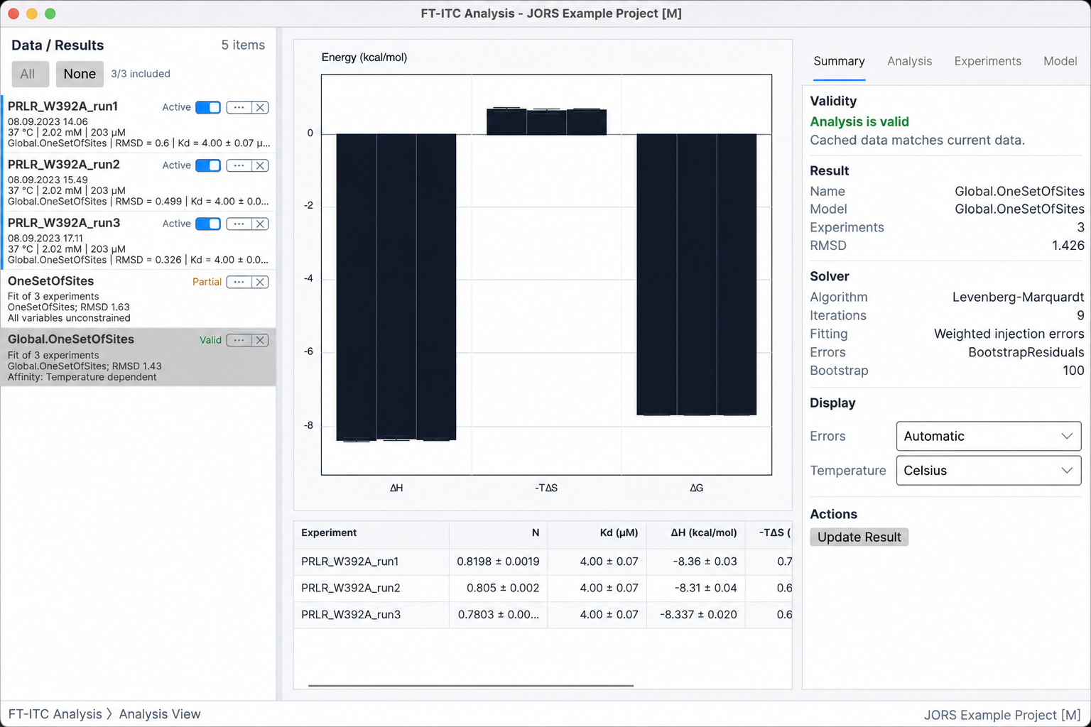
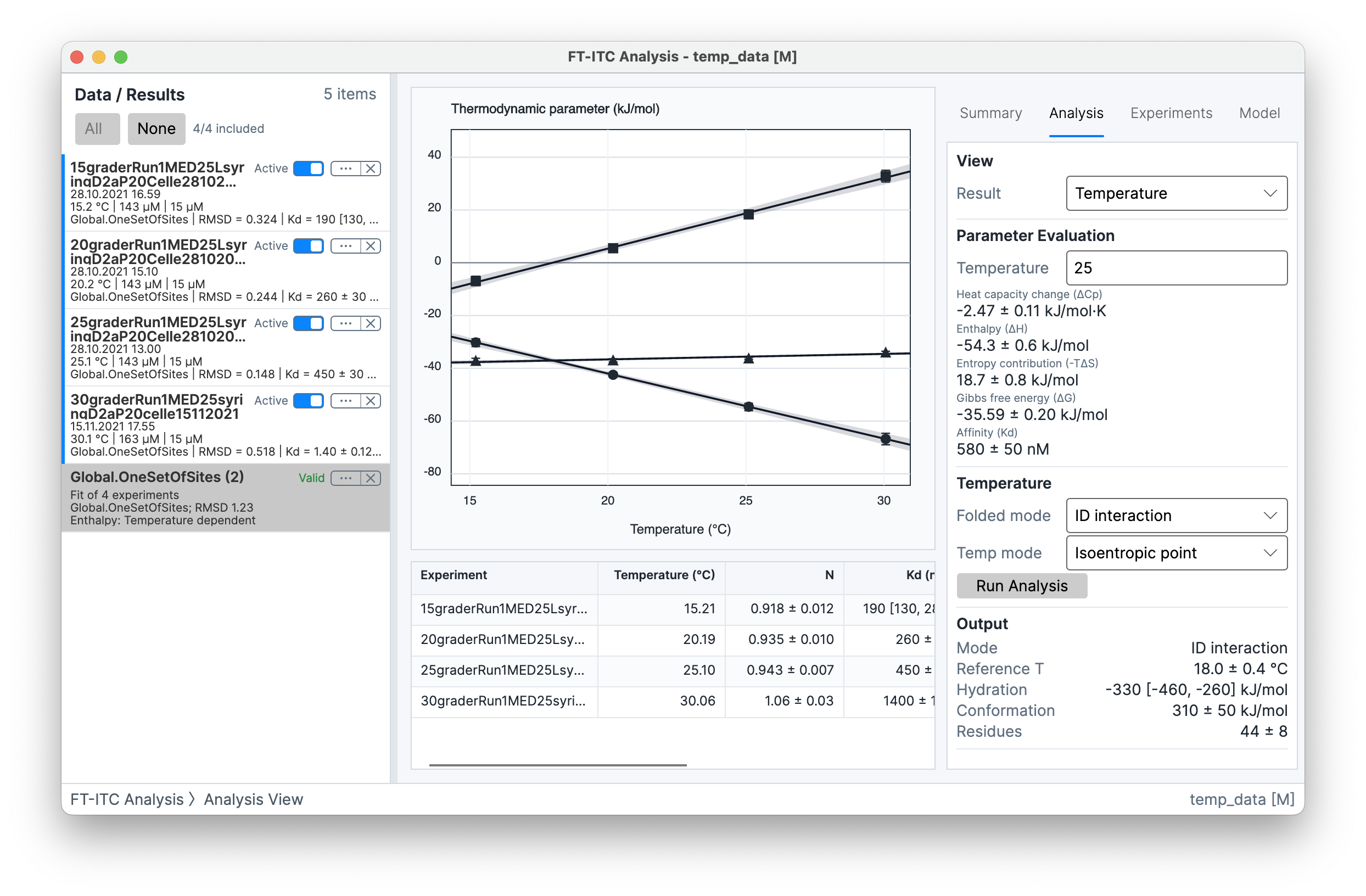
The Analysis tab contains the result view selector, parameter evaluation, and the analysis-specific controls and outputs. It is also the location of the uncertainty display, correlation information, and evaluation-temperature presentation associated with the selected view. Energy labels and values use the family resolver for the visible central-value group, including graph axes, errors, fitted bands, tooltips, and parameter lists.
The Experiments tab lists the result members and their stored status and condition information, including member temperature. The member represented as selected in the result table drives Fit, while this tab provides the corresponding member context.
The Model tab shows the stored model options, locked parameters and their fixed values, and the active constraints. A constraint with state None is not listed as an active global constraint; Same for all and Temperature dependent entries identify the relationships retained by the Analysis Result. The corresponding labels Independent and Shared describe the same member-specific and common relationships.
Uncertainty and evaluation temperature
The Errors display control provides Automatic, Standard deviation, 95% confidence interval, and SD + 95% CI. Standard deviation presents the primary best-fit value with a symmetric ± SD; 95% confidence interval presents that same best-fit value with the lower and upper percentile limits; and SD + 95% CI presents both. The central value is always the primary best fit, not the mean or median of the resampled values.
Automatic makes this choice separately for each reported quantity. Let L and U be its stored 95% confidence limits and θ̂ its primary best-fit value:
The decision is made after a fitted coordinate has been transformed into the displayed quantity. A nonlinear transformation—such as fitting log10(Ka) and displaying Kd—can therefore make the displayed interval asymmetric and cause Automatic to select CI for that quantity.
Changing Errors changes only how stored uncertainty is presented in tables, parameter evaluation, and graphs. It does not rerun the fit, change the best-fit parameters, or turn one error-estimation method into another. Bootstrap construction, parameter transformation, and the SD and percentile calculations are described under Parameter uncertainty.
The Parameter Evaluation section contains an evaluation Temperature field and the displayed thermodynamic quantities at that temperature. Temperature display can be Celsius or Kelvin. Changing the evaluation temperature changes derived presentation from the stored model; it does not change injection heats or refit the result. Temperature-dependent values are meaningful together with their model, units, uncertainty representation, and evaluation temperature.
Parameter correlation
Correlation shows Pearson correlations between fitted parameter coordinates across residual-bootstrap refits. It requires Bootstrap residuals, at least 30 complete refits, and at least two parameters that vary across those refits. Parameters with no variation are omitted. Parameters fixed in the primary fit are also omitted unless Unlock parameters allowed them to vary during bootstrap error estimation; such parameters are marked with an asterisk and a warning that bootstrap parameter unlocking was enabled.
For each off-diagonal cell, the application also reports an approximate 95% Monte Carlo precision interval using Fisher's transformation. Matrix values range from −1 to +1; an interval spanning zero marks the sign as unresolved at the current simulation precision. The result panel separately reports attempted, usable, failed, and complete refits. It warns when fewer than 100 complete refits make precision coarse, at least 20% of attempted refits failed, a usable refit lacked a finite displayed coordinate, a sign is unresolved, or the matrix is structurally rank limited. The correlation matrix remains unavailable below 30 complete refits. For a single-experiment result, the scope is Single experiment. A multiple-experiment result can show Shared coordinates alone or Shared + selected local coordinates when a member is selected. Shared and local labels identify the scope of each parameter.
Sequential correlations use the actual fitted coordinates. Affinity coordinates are labeled log10 Ka1 through log10 Ka4, active enthalpy coordinates are included, and no N-value coordinate is added. A global result shows the shared per-step coordinates and, when requested, unconstrained coordinates for the selected member without duplicating constrained member values.
Advanced analysis views
All advanced analyses require a One-Set-Of-Sites Analysis Result. Availability is additionally conditional on the relevant condition span and metadata. The advanced analyses operate on the stored member solutions and expose their own calculated outputs; they do not change the base fit parameters. A sequential result can still show its ordinary per-step ΔH, ΔG, −TΔS, Kd, and temperature-dependence presentation; it reports the Spolar Record method, protonation, and electrostatics as unsupported by that model rather than hiding the ordinary thermodynamic views.
Temperature
The Temperature view is available when member temperatures span more than the configured minimum temperature span. Its temperature-analysis controls expose Folded mode values Globular and ID interaction, together with Temp mode values Isoentropic point, Mean temperature, and Reference temperature.
The stored temperature-analysis output includes reference temperature, hydration contribution, conformational contribution, and residue estimate. These values describe the selected folded and temperature-evaluation modes under the fitted temperature dependence. They remain conditional estimates of the stored model and member series rather than direct structural measurements.
Salt
The Salt view requires a Salt attribute for every member and sufficient ionic-strength span across the member set. Its Graph mode values are Affinity vs Salt, Debye-Huckel, and Counter Ion Release. Counter-ion release is a salt analysis mode and is presented in the Salt view rather than as a separate advanced analysis.
The Salt output includes the extrapolated Kd0 and Counter ion result when the analysis has a calculated fit. The graph mode determines whether the displayed dependence is expressed against salt, ionic strength using Debye-Huckel behavior, or ion activity for counter-ion release. The result is limited by the recorded salt identities, ionic-strength values, and the quality and span of the member affinity values.
Protonation
The Protonation view requires a Buffer attribute for every member and at least two distinct buffer identities. Its calculated output contains Protons and Binding H, with uncertainty when the stored analysis contains the corresponding uncertainty results.
The view relates the stored member binding enthalpies to the buffer protonation information associated with their conditions. The result is conditional on the recorded buffer identities, their temperature-dependent protonation enthalpies, and the model assumptions; it does not identify a particular residue or microscopic protonation event.
Advanced-analysis values are supplemental views of a stored Analysis Result. Their availability and outputs are determined by the One-Set-Of-Sites model, member variation, metadata, selected graph or evaluation mode, and any completed uncertainty calculation. Result validity remains a separate indication of whether the stored fit inputs match the current project state. Figure and table output is covered in Figures and export.
Independent reference checks for temperature, protonation and electrostatic calculations are listed in the scientific evidence matrix. They check units, central values and selected source constants; they do not establish interval coverage or the physical adequacy of the selected interpretation. The buffer registry contains approximations and some unknown quantities, so confirm that the chosen buffer values apply to the experiment. The source-checked TAPSO pKa temperature correction is a local approximation validated over 20–30 °C. Its protonated zwitterion is neutral, and imidazole's ionization heat-capacity slope is −9 J/(mol K). Recalculate affected derived analyses when comparing with results produced before these corrections.