
Processing
Baseline models, integration regions, injection uncertainty, and processing propagation and locking.
Last verified:
The Process Data workspace estimates and subtracts a baseline from the differential-power trace, integrates the corrected response for each injection, and estimates an uncertainty for the resulting heat. Polynomial and Segmented baselines provide repeatable, model-based treatment with less manual shaping when their assumptions suit the trace. Spline-point editing provides precise local control for difficult cases, while graphical boundary editing, Fit Peaks, and copying between injections accelerate integration-region adjustment.
These controls make processing efficient without deciding the scientific interpretation for you. Confirm that the chosen baseline represents the signal between injections and that each integration region captures the observed response.
Raw .itc, .nitc, .ta, and .apj imports use this workflow, as do Origin .opj imports that contain a usable time/power trace. Integrated-heat imports and Origin projects without a usable trace skip Process Data.
Processing workspace
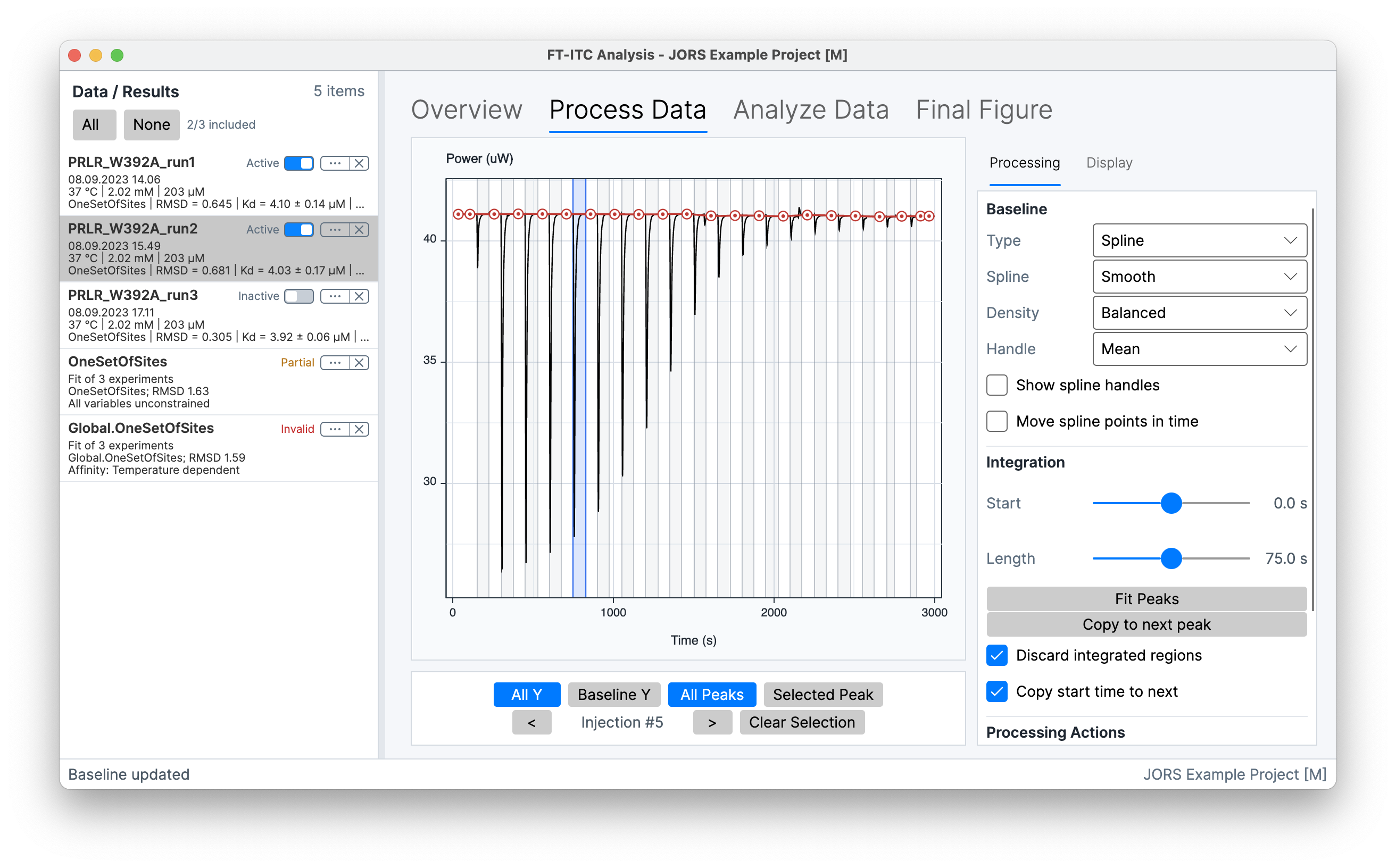
The Processing controls configure the baseline and integration regions. The Display controls show or hide the baseline, integration regions, corrected data, and cursor information.
With All injections selected, Start and Length apply to every injection. A selected graph region targets one injection, and double-clicking it focuses the graph on that peak. The previous and next controls move through the injections; Clear Selection returns to all injections.
The view controls separate horizontal and vertical scaling:
- All Y shows the complete power range, while Baseline Y emphasizes the baseline region.
- All Peaks shows the full injection series, while Selected Peak focuses on the current injection.
- Dragging an empty part of the graph zooms into the selected region.
Baseline models and editing
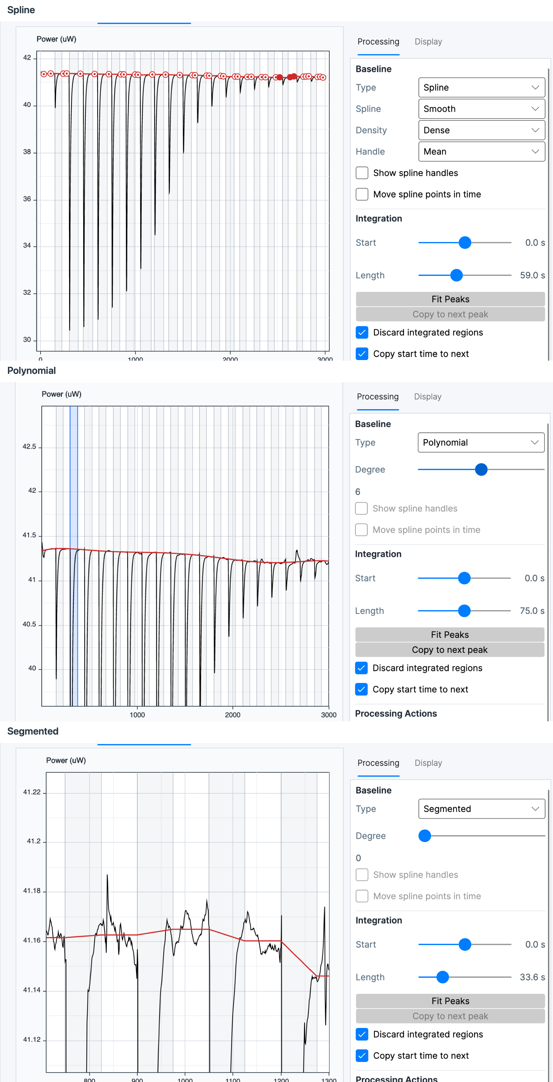
Spline
Spline places points in usable baseline regions and interpolates between them. It provides the most direct graphical control.
- Linear connects the spline points with straight sections. Smooth produces a continuously varying baseline and supports editable slope handles.
- Sparse, Balanced, and Dense change the number of automatically generated points.
- Mean, Median, and Min volatility determine the representative power used for an automatically generated point.
- Show spline handles displays the slope handles for a Smooth spline. Move spline points in time allows a point to be dragged horizontally as well as vertically.
Dragging a point corrects its position. A secondary-click on the graph adds a point At Data or At Baseline. A secondary-click on an existing point exposes Lock or Unlock, Mark Linear or Unmark Linear, and Remove. Marking neighboring points as linear makes the interval between them straight. Locked points are retained when automatic spline points are regenerated.
Balanced provides the middle spline-point density. Greater density increases local flexibility but can also follow noise or absorb part of an injection response.
Polynomial
Polynomial fits one polynomial across the complete thermogram and is suited to smooth global drift. Degree controls flexibility.
Polynomial behavior is least constrained at the beginning and end of the run, where a high degree can produce strong edge behavior. Additional degree increases flexibility whether it represents baseline drift or follows more of the trace.
Segmented
Segmented fits local constant, linear, or quadratic baseline behavior between integration regions and blends the local estimates across the run. It is suited to locally changing drift for which one global polynomial is too rigid. Degree selects the local behavior.
Local flexibility can follow genuine drift, but it also makes the result more dependent on the integration boundaries and on the baseline immediately around each peak.
Exclude integration regions from the baseline
When Discard integrated regions is enabled, data inside the current integration regions are excluded when the baseline is recalculated. Moving a boundary can therefore change both the integrated area and the estimated baseline.
Convert to a spline
A Polynomial or Segmented baseline can be converted to a Smooth or Linear Spline when the automatic baseline is a useful starting point for graphical editing. Conversion changes the baseline representation and creates editable spline points.
Integration regions
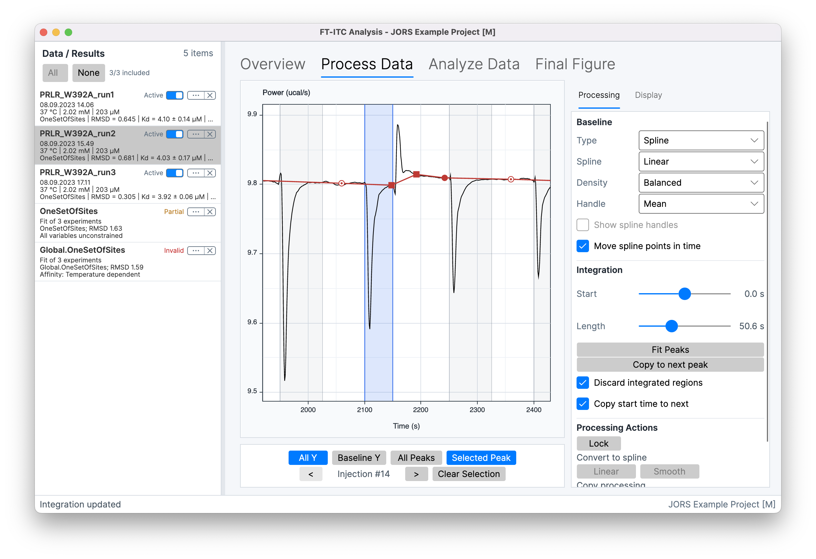
Each injection region has a start and an end boundary. Start sets the offset of the start boundary relative to the injection. The value displayed as Length positions the end boundary that many seconds after the injection begins; it is not a separate processing mode.
Either boundary can be dragged in the graph or adjusted with the controls. The application constrains the start and end to a valid interval within the injection scope and preserves a minimum separation between them.
Estimate end points with Fit Peaks
Fit Peaks estimates the end point of each injection from the decay of the baseline-corrected response. It changes the end boundaries and then integrates the resulting regions; it does not fit the integrated heats or select a persistent integration mode.
When peak fitting converges, the estimated boundaries replace the previous end points. If fitting fails or does not converge, the previous regions remain unchanged. Peak kinetics can vary across the titration, and the first injection can behave differently from the remaining series.
Copy a region to the next injection
Selecting an injection and choosing Copy to next peak, or pressing Space, copies its end boundary and advances to the next injection. Copy start time to next includes the start boundary in that operation.
Injection uncertainty
Each injection error bar represents an estimated ±1 standard deviation for that injection's molar heat. The estimate describes how local noise in the baseline-corrected thermogram propagates through the selected integration region. It is calculated independently for every injection, so the bars can vary across a titration.
The calculation uses baseline-corrected samples around the injection. It combines an estimate of local power noise with the temporal correlation between neighboring samples, the integration-region length, and uncertainty in the baseline level. A longer or noisier region will therefore often have a larger estimated uncertainty. When Buffer Subtraction is applied, the independent target and reference heat uncertainties are combined.
The bars do not include uncertainty in cell or syringe concentration, fitted parameters, or model-derived confidence bands. They also do not quantify baseline-model choice, integration-boundary choice, calibration error, other instrumental effects, or other systematic uncertainty. Consequently, they do not validate the selected processing or constitute confidence intervals for the true heat.
Weight by injection error can use these estimates in the fitting objective. Concentration uncertainty is handled separately in supported resampling calculations. Both behaviors are described under Fitting calculation.
Propagate and lock processing
Active under Copy processing copies the selected experiment's processing to the other Active experiments. This can replace existing processing when a destination is unlocked. New targets experiments that do not yet have processing.
Processing can be propagated while the source is unlocked. Locked destinations are not overwritten. After propagation, each processor that should be protected can be selected and set to Lock. Locking disables baseline, spline-point, integration-region, and peak-fitting edits; Unlock makes changes available again.