Single-experiment fitting

Fit one experiment, configure model and uncertainty options, control injection inclusion, and interpret fit diagnostics.

Last verified: 2026-08-26

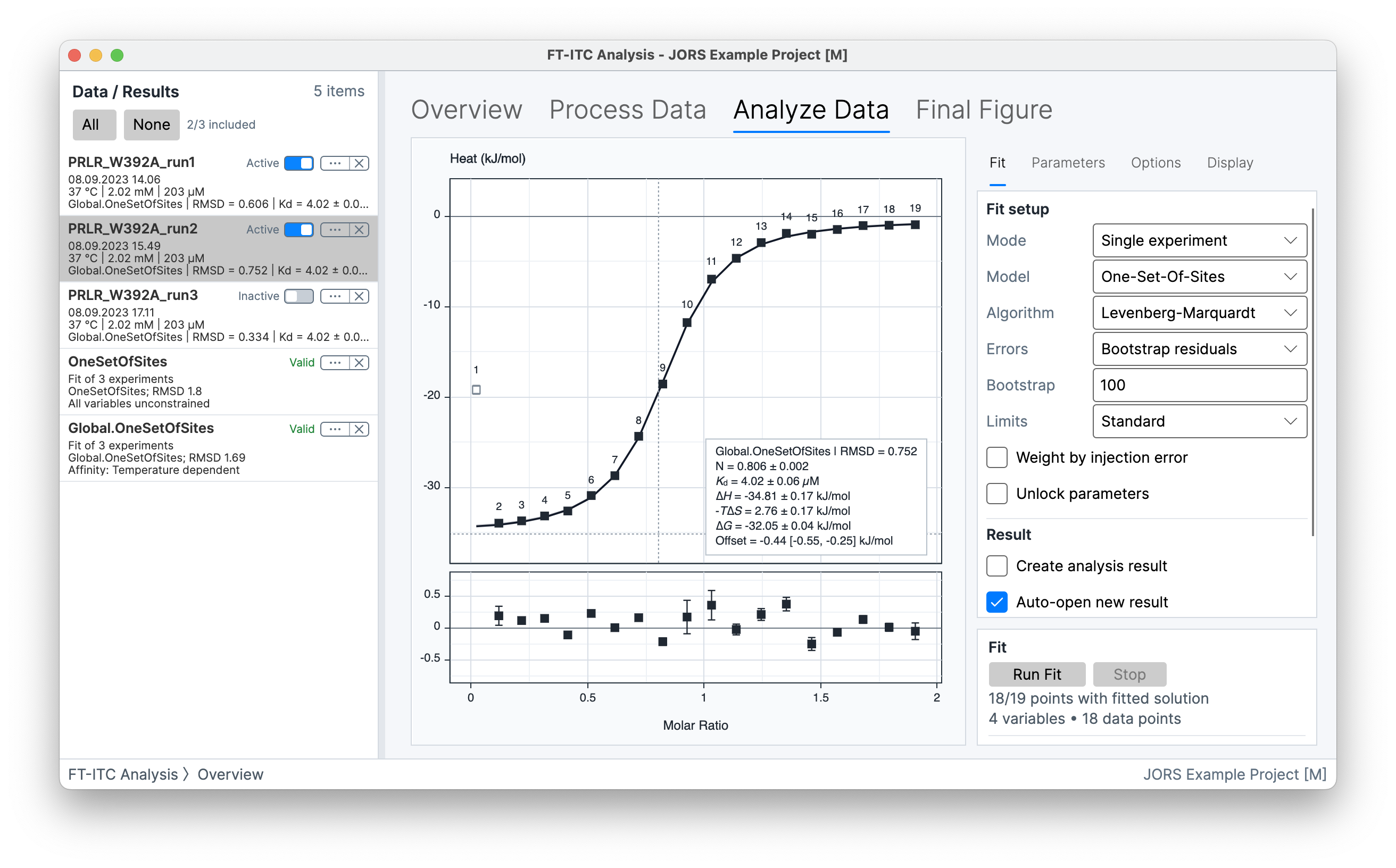
Analyze Data in Single experiment mode fits the integrated heats of the selected Experiment Data. The fit uses the included injections together with the experiment concentrations, injection volumes, cell volume, temperature, and any model-specific information.

The inspector has four tabs:

• Fit selects the model, optimizer, error-estimation method, limits, weighting, and result output.
• Parameters shows the model parameters and their starting or fixed values.
• Options contains settings specific to the selected model.
• Display controls the fitted curve and diagnostic information shown in the graph.

Profile-likelihood uncertainty

Profile likelihood is a fixed-95% uncertainty method. After a successful primary fit, one fitted coordinate at a time is fixed while nuisance coordinates are refit. Unweighted fits use an F-calibrated RSS interval assuming independent Gaussian residuals; weighted fits use a one-degree-of-freedom chi-square increment conditional on the supplied peak-area SDs. The primary fit remains the reported value.

Integration graphs can display the envelope from available leave-one-out refits (typically a small ensemble); profile likelihood creates no refit ensemble or confidence band.

An endpoint is reported only when both sides cross the threshold. Reaching a parameter limit is computational censoring, not a confidence endpoint, so that side remains unavailable. The displayed value ± SD uses an explicitly equivalent symmetric scale computed from the asymmetric profile interval; it is not a Gaussian sample standard deviation. Save profile results as FTXTC to preserve the profile run diagnostics.

Multiple-experiment fitting uses additional experiment selection and parameter constraints; see Multiple-experiment fitting.

Injection inclusion

Selecting an injection point in the integrated-heats graph changes whether it is included in the fit. Excluded injections do not contribute to the objective function. The Excluded points option in Display keeps excluded injections visible and available for selection.

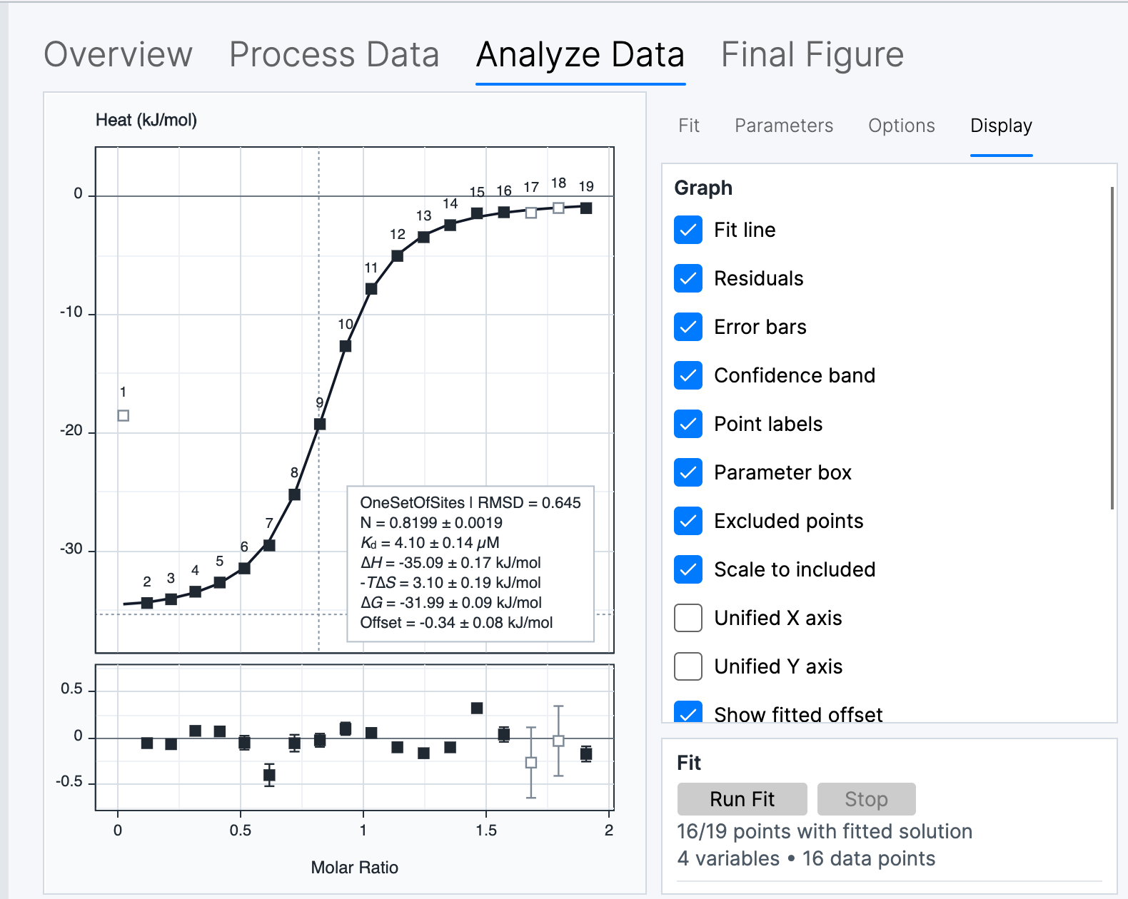
Changing injection inclusion does not rerun the fit. The fitted curve and parameters continue to represent the previous fit until Run Fit is used again. An inclusion change can also invalidate an Analysis Result that contains the experiment.

Models

One-Set-Of-Sites

One-Set-Of-Sites represents one class of equivalent, independent binding sites. It fits stoichiometry, dissociation constant, binding enthalpy, and an injection-heat offset. The solution also reports thermodynamic quantities derived from the fitted affinity and enthalpy.

The Options tab provides Use Syringe Correction and Stoichiometry. Without syringe correction, the fitted N-value represents the apparent site stoichiometry. With syringe correction enabled, Stoichiometry fixes the number of cell-side sites and the fitted N parameter becomes the active syringe-concentration factor alpha.

The model cannot by itself distinguish a concentration error from other effects that change an apparent stoichiometry.

Two-Sets-Of-Sites

Two-Sets-Of-Sites represents two independent classes of sites. It fits separate stoichiometries, dissociation constants, and enthalpies for the two classes, together with a shared injection-heat offset.

Shared N-Values makes the two site classes use the same fitted stoichiometry. Use Syringe Correction instead fixes the first and second Stoichiometry values and fits one active syringe-concentration factor, alpha.

The two site labels are interchangeable: exchanging all parameters assigned to site 1 and site 2 describes the same physical model. A lower fitting loss alone does not establish that two distinguishable binding processes are supported by the experiment.

Sequential Binding Sites

Sequential Binding Sites represents two, three, or four ordered binding steps on a macromolecule in the cell. Sequential binding steps in the Options tab selects the fixed integral step count. The model fits one macroscopic stepwise association constant and one molar step enthalpy for each transition, together with the ordinary molar injection-heat offset. It does not fit an N-value or syringe activity.

For step count n, let β₀ = 1, β_i = ∏_j=1…iK_j, and let x be free ligand. The state weights and fractions are

Here M_t and X_t are total macromolecule and ligand concentrations in the cell. The model solves the ligand balance internally and calculates the cell heat content from the population of every sequential state:

The reported K_i values are phenomenological, macroscopic step constants for the ordered transitions M → MX → MX₂ and so on. They are not microscopic intrinsic site constants. Step numbers therefore have physical order and fitted steps are never sorted or treated as exchangeable.

The macromolecule must be in the cell and ligand in the syringe. Reverse titrations with macromolecule in the syringe are outside this model. Multi-step fits can be weakly identifiable, especially when the concentration window does not populate every transition. Inspect parameter bounds, residuals, bootstrap uncertainty, and parameter correlations; an improved RMSD does not by itself establish the selected number of sequential steps.

Competitive Binding

Competitive Binding represents titration of a target ligand into a macromolecule that is initially in equilibrium with a prebound ligand in the cell. It fits the target ligand's stoichiometry, dissociation constant, binding enthalpy, and injection-heat offset.

The Options tab requires the prebound ligand [Ligand], Ligand Affinity, and Ligand Enthalpy. From attributes makes [Ligand] use the corresponding value stored in the Experiment Data attributes instead of the value entered in the model options. The model also provides Use Syringe Correction and Stoichiometry with the same concentration-factor interpretation as One-Set-Of-Sites.

The fitted target affinity and enthalpy depend on the supplied prebound-ligand properties. Those values are model inputs rather than quantities independently determined by the competitive fit.

Dissociation

Dissociation represents dilution-driven monomer-dimer self-association. The syringe contains the macromolecule and the cell initially contains buffer. Dilution and mixing change the dimer population, and the model fits the association equilibrium through its reported dissociation constant, the association enthalpy per mole of dimer formed, and an injection-heat offset.

This is not a general model for dissociation of an arbitrary preformed complex or for other oligomerization schemes. It has no stoichiometry or syringe-correction options.

Thermodynamic relationships

The application derives thermodynamic quantities from the fitted affinity and enthalpy. Temperature T is expressed in kelvin.

Parameters and model options

The application's scientific evidence matrix separates published-data comparisons, independent synthetic references and diagnostic cases. It includes a reproducible raw thermogram-to-result example and independent full-fit references for the binding and dissociation models. These examples validate stated equations, units and numerical settings. They do not establish that every parameter is identifiable in a particular noisy experiment. Higher-step synthetic recovery uses documented tighter numerical settings; a small RMSD alone does not establish parameter accuracy.

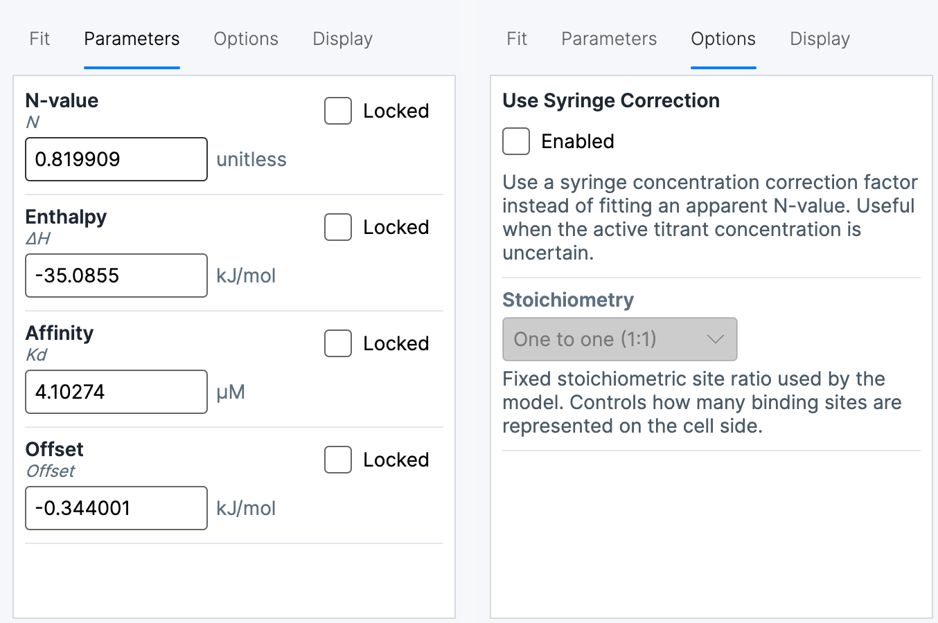
The application generates initial parameter values from the experiment and can reuse an attached fitted solution where applicable. Entering a value replaces the generated starting value for that parameter. Values are displayed in the current application units. Clearing a value returns the parameter to automatic initialization.

Locked holds a parameter at its displayed value during the primary fit. An unlocked parameter is adjusted by the optimizer. Locked values remain part of the model and affect every other fitted parameter even though they are not estimated by that fit.

Analysis choices are retained separately for the available fitting modes and models. Restore defaults clears the stored analysis inputs and reloads the live inspector fitting controls from the current Preferences. It also resets inspector-only parameter unlocking. The action does not change Preferences or preference-backed limits, result-output, and display settings.

The Limits control selects a common parameter-bound policy:

• Standard uses the normal parameter bounds.
• Expanded permits a wider parameter range.
• No limits removes the configured parameter bounds.

A fitted value at a bound is not an interior estimate. It indicates that the reported value depends on the selected bound as well as on the data and model.

Before a fit starts, the application checks every free starting parameter against the currently selected limits. This includes values entered manually, values reused from an attached solution, and automatic values that become stale after the Limits policy changes. Bounds are inclusive, so a value exactly at a bound is allowed. Locked and globally determined parameters are not checked because they are not optimizer coordinates. An out-of-range value is marked in the Parameters inspector and Run Fit remains available so it can be corrected. The fit is blocked with a list of affected parameters; edit the value, clear it to restore the automatic default, or widen Limits. In a global fit, a local parameter that has no exposed global editor is identified by its experiment name in the fit status area; edit that experiment in single-experiment mode if needed.

Fitting calculation

Algorithm

Levenberg-Marquardt uses local derivative information and can be efficient when the starting values describe a suitable region of the fitting surface.

Nelder-Mead is a derivative-free simplex optimizer. It provides an alternative calculation for surfaces or starting conditions that are less cooperative for the local derivative-based method. Agreement between optimizers does not by itself establish that the selected model is scientifically adequate.

Weight by injection error

Weight by injection error uses the integration uncertainty estimated during thermogram processing when calculating the fitting objective. Injections with larger estimated uncertainty consequently have less influence than injections with smaller estimated uncertainty.

The displayed RMSD is always calculated from the unweighted residuals, including after a weighted fit. It therefore remains distinct from the weighted objective minimized by the optimizer.

For a multiple-experiment result, the displayed global RMSD is pooled across every included injection in every member experiment. Each member row retains its own local RMSD, so the global value remains comparable when members contain different numbers of included injections.

If an included injection does not have a finite positive peak-area SD, the application uses the mean of the finite positive SD values from the other included injections. If none is available, it uses a small numerical fallback so the calculation remains defined. A substituted value prevents division by zero; it does not turn a missing processing estimate into a measured uncertainty.

The weighting describes the application's processing-derived uncertainty model. It does not account for every systematic source of experimental or processing uncertainty.

Parameter uncertainty

The Errors control determines whether the primary best fit is followed by repeated refitting:

• None retains the primary fit without resampling-based parameter uncertainty.
• Bootstrap residuals standardizes each included injection's primary-fit residual by the same effective peak-area SD described above, centers that standardized pool, samples independently with replacement, rescales each draw by the target injection's effective SD, and adds it to the best-fit prediction. The synthetic injection retains the target injection's stored peak-area SD; when error weighting is enabled, the refit therefore uses the same per-injection weighting inputs and fallback rule.
• Leave-one-out performs one deterministic refit for each deletion: one refit per included injection in a single-experiment analysis, or one refit per omitted experiment in a globally fitted multiple-experiment analysis. Concentrations, uncertain model options, and parameter locks are held at their primary-fit values so the resulting spread isolates deletion sensitivity.
• Profile likelihood fixes each fitted coordinate in turn and refits nuisance coordinates against the conditional likelihood. It uses the local objective for independent members and the complete objective for shared global coordinates; complete asymmetric crossings are retained as endpoints, while a bound reached before crossing is reported as censoring.

Bootstrap sets the requested number of residual-bootstrap iterations. It is enabled and used only for residual bootstrap; leave-one-out and profile likelihood have deterministic schedules and do not use this count. Only included injections supply residuals, and only retained usable refits enter the parameter distributions. Because residual-bootstrap sampling is with replacement, one residual can occur more than once in a synthetic dataset while another may not occur at all. The fit status distinguishes successful and failed refits.

Correlation diagnostics distinguish attempted refits, optimizer-usable refits, and the listwise-complete refits whose displayed coordinates are all finite. A high failed-refit fraction can make the retained ensemble selective; increasing the requested count improves Monte Carlo resolution but does not correct a systematically failing refit process.

Each replicate uses a fresh independent random stream; seeds are not stored, so rerunning a bootstrap does not reproduce the same random sequence.

When Update Result is used on a stored residual-bootstrap Analysis Result, its dialog shows the retained usable-refit count and offers the stored behavior plus larger supported presets up to 10,000 requested iterations. The update performs a fresh complete fit and bootstrap; it does not append samples to the saved distribution. Cancelling the calculation or completing it without any usable bootstrap refits preserves the previous Analysis Result.

The primary best-fit parameter remains the reported value. For a parameter with best-fit value θ̂ and values θ_b from B retained refits, the application summarizes the bootstrap distribution as follows:

The uncertainty display can show SD, the 95% confidence interval, both, or select between them automatically. This presentation rule is described under Uncertainty and evaluation temperature.

Concentration uncertainty

With Concentration uncertainty enabled in the Fit tab, the concentration SDs entered in Details... are propagated through residual-bootstrap calculations. The control is initialized from the corresponding preference and is active only for residual bootstrap; leave-one-out and profile likelihood keep primary concentrations fixed. Each nonzero fractional SD is the arithmetic standard deviation relative to the entered concentration. Synthetic clones draw a positive, mean-preserving lognormal multiplier: if the fractional SD is c, then σ²_log = ln(1 + c²), μ_log = −σ²_log/2, and the multiplier is exp(μ_log + σ_logZ) for a standard-normal Z. Thus the multiplier has mean 1 and SD c, so cloned concentrations remain positive while preserving the entered arithmetic mean and SD. Explicit cell or syringe SDs take precedence over the automatic value configured in Preferences. These uncertainties affect the synthetic experiment concentrations used for bootstrap refits, not the concentrations used for the primary best fit.

Displayed parameter uncertainty

The bootstrap summary is first calculated for each fitted parameter coordinate. The application then converts that summary into the quantity shown to the user. For example, affinity is fitted as log₁₀(K_a) but is normally displayed as K_d. The displayed central value comes from the primary best fit, SD is propagated through the transformation, and the percentile limits are transformed and reordered as required.

Quantities calculated from more than one reported parameter, such as −TΔS, use the application's uncertainty-propagation rules for that calculation. Their displayed limits are therefore not necessarily the percentiles that would be obtained by recalculating the complete derived quantity independently for every bootstrap refit. The Automatic SD-or-CI decision is applied after transformation or propagation, separately for each displayed quantity.

Unlock parameters during error estimation

Locked parameters remain fixed during the primary fit. With Unlock parameters enabled, copies of those parameters are unlocked only for residual-bootstrap refits and can vary in the resampled solutions. Leave-one-out and profile likelihood always preserve the primary-fit locks.

This setting does not change or rerun the primary best fit. It changes only the parameter state used by the repeated error-estimation fits, and it has no effect when no fitted parameter is locked.

Fit execution and diagnostics

Run Fit starts the primary optimization and the selected error-estimation calculation. Stop requests cancellation of the active calculation. When fitting ends, the status reports the termination state, RMSD, iteration count, and elapsed time. A resampling calculation also reports its outcome and the number of successful and failed refits.

The Display tab exposes complementary diagnostics:

• Fit line shows the curve calculated from the current fitted solution.
• Residuals show the difference between each included observation and the fitted curve.
• Error bars show the processing-derived integration uncertainty.
• Confidence band shows uncertainty around the fitted curve when the solution contains suitable resampling results.
• Excluded points shows injections that do not contribute to the current fit.

These displays describe different aspects of the fitted solution. A small RMSD does not rule out systematic residual structure, poorly identified parameters, or dependence on model assumptions.

Store the fitted solution

With Create analysis result disabled, a successful single-experiment solution remains attached to its Experiment Data and is available in that experiment's analysis and figure workflows.

With Create analysis result enabled, a usable completed fit also creates a separate Analysis Result containing the experiment, model, fit settings, and solution. Auto-open new result determines whether the new result workspace opens immediately. A stopped or unusable fit does not create or replace an Analysis Result.

Fit availability and non-convergence

A single-experiment analysis requires processed or imported heats and at least three included injections with usable numerical values. The binding models also require nonzero cell and syringe concentrations. Dissociation uses the syringe concentration and does not require a macromolecule concentration in the initially buffered cell.

An unavailable model, failed termination, bound-limited solution, or failed resampling population can reflect missing or degenerate heat and concentration information, the supplied starting values, the selected limit policy, the optimizer's interaction with the fitting surface, model complexity, or weak parameter identifiability. Resampling can fail even when the primary fit succeeds because each refit presents a different or reduced dataset to the same model.